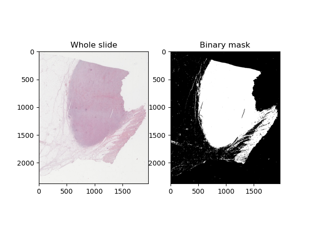
Project Computer Vision – Image Analysis and Enhancement of Histopathology Slides

Whole slide image (Level 3, width and height decimation by 32)

Central slice of whole slide image (height,width) = (300 , 400)

Visualization of stain vector estimation

Stain de-convolution

Method 1 : least square fitting

Solve the linear equation Ax = b,

where A is the estimated stain vectors, b is optical density(OD).

# Method 1 : least squared fitting
A = stainVectors.T
b = np.reshape(OD,(ROI_height*ROI_width,3)).T
x, _, _, _ = np.linalg.lstsq(A,b)
hema_lstsq = np.reshape(x[0,:],(ROI_height,ROI_width))
eosin_lstsq = np.reshape(x[1,:],(ROI_height,ROI_width))

Method 2 : Moore-Penrose pseudo-inverse

# Method 2 : Moore-Penrose pseudoinverse
inv_matx = np.linalg.pinv(np.dot(stainVectors,stainVectors.T))
result = np.dot(np.dot(OD,stainVectors.T),inv_matx)
hema = result[:,:,0]
eosin =result[:,:,1]